This blog post was written in a Jupyter notebook.
Click here for an interactive version:
![]()
Modeling Coronal Loops in 3D with sunpy.coordinates#
Will Barnes is a fifth-year PhD student in the Department of Physics and Astronomy at Rice University in Houston, TX, USA. Will is a frequent user of the SunPy package and is the developer of fiasco, a Python interface to the CHIANTI atomic database. You can find him on GitHub @wtbarnes and Twitter @wtbarnes_.
Updated on 25 July 2018
The first version of this post contained an error in the scaling laws used to compute the loop temperature from a heating rate. This has now been corrected.
Coronal loops are the building blocks of the solar corona, the outermost layer of the Sun’s atmosphere. Because the pressure exerted by the coronal magnetic field is much stronger than the pressure of the surrounding gas, hot plasma is forced to flow along the magnetic field lines, creating bright arches, or loops, that extend high above the solar surface. As a result, the corona is often modeled as an ensemble of one-dimensional loop structures rather than a three-dimensional box of magnetized plasma. This allows for detailed simulations over massive spatial scales that are not accessible by 3D MHD simulations due to their massive computational cost. This review paper provides an excellent overview of both the observational and modeling sides of coronal loop physics.
The sunpy.coordinates module is a useful tool for expressing locations on the Sun in various coordinate systems. While most often used in the context of analyzing and manipulating observational data, we can also use this module to build three-dimensional models of loops in the corona.
Getting the Coordinates of a Single Loop#
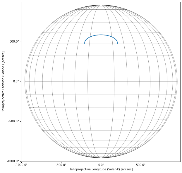
Let’s consider a semi-circular loop with both footpoints rooted on the surface of the Sun with a length \(L=500\) Mm and centered at a latitude of \(\Theta=30^{\circ}\). We have to do a bit of algebra to find these coordinates, but all we are doing is expressing them in terms of a spherical coordinate system, more specifically the Heliographic Stonyhurst coordinate system, \((r,\Theta,\Phi)\). For a comprehensive overview of solar coordinate systems, see Thompson (2006).
[2]:
def semi_circular_loop(length, theta0=0 * u.deg):
    r_1 = const.R_sun

    def r_2_func(x):
        return np.arccos(0.5 * x / r_1.to(u.cm).value) - np.pi + length.to(u.cm).value / 2.0 / x

    r_2 = scipy.optimize.bisect(r_2_func, length.to(u.cm).value / (2 * np.pi), length.to(u.cm).value / np.pi) * u.cm
    alpha = np.arccos(0.5 * (r_2 / r_1).decompose())
    phi = np.linspace(-np.pi * u.rad + alpha, np.pi * u.rad - alpha, 2000)
    # Quadratic formula to find r
    a = 1.0
    b = -2 * (r_1.to(u.cm) * np.cos(phi.to(u.radian)))
    c = r_1.to(u.cm) ** 2 - r_2.to(u.cm) ** 2
    r = (-b + np.sqrt(b**2 - 4 * a * c)) / 2 / a
    # Choose only points above the surface
    i_r = np.where(r > r_1)
    r = r[i_r]
    phi = phi[i_r]
    hcc_frame = Heliocentric(observer=SkyCoord(lon=0 * u.deg, lat=theta0, radius=r_1, frame="heliographic_stonyhurst"))
    return SkyCoord(
        x=r.to(u.cm) * np.sin(phi.to(u.radian)),
        y=u.Quantity(r.shape[0] * [0 * u.cm]),
        z=r.to(u.cm) * np.cos(phi.to(u.radian)),
        frame=hcc_frame,
    ).transform_to("heliographic_stonyhurst")
[3]:
loop = semi_circular_loop(500 * u.Mm, theta0=30 * u.deg)
[4]:
loop[[0, -1]] # First and last points
[4]:
<SkyCoord (HeliographicStonyhurst: obstime=None): (lon, lat, radius) in (deg, deg, km)
    [(-14.09138695, 29.2478234, 698633.18692374),
     ( 14.09138695, 29.2478234, 698633.18692374)]>
Notice that this function returns an Astropy SkyCoord object. You can read more about these in the Astropy docs. Simply put, a SkyCoord object allows us to specify a coordinate-aware set of points in the sky, specifically on the Sun. SunPy provides many of the commonly used solar coordinate systems to be used by SkyCoord. You can read more about them
here.
To plot our loop, we need to construct a dummy sunpy.map.Map object. This just provides a projected coordinate system so that we can plot our loop in two dimensions.
[5]:
data = np.ones((10, 10))
time_now = astropy.time.Time.now()
meta = MetaDict(
    {
        "ctype1": "HPLN-TAN",
        "ctype2": "HPLT-TAN",
        "cunit1": "arcsec",
        "cunit2": "arcsec",
        "crpix1": (data.shape[0] + 1) / 2.0,
        "crpix2": (data.shape[1] + 1) / 2.0,
        "cdelt1": 1.0,
        "cdelt2": 1.0,
        "crval1": 0.0,
        "crval2": 0.0,
        "hgln_obs": 0.0,
        "hglt_obs": 0.0,
        "dsun_obs": const.au.to(u.m).value,
        "dsun_ref": const.au.to(u.m).value,
        "rsun_ref": const.R_sun.to(u.m).value,
        "rsun_obs": ((const.R_sun / const.au).decompose() * u.radian).to(u.arcsec).value,
        "t_obs": time_now.iso,
        "date-obs": time_now.iso,
    }
)
dummy_map = GenericMap(data, meta)
[6]:
fig = plt.figure(figsize=(10, 10))
ax = fig.gca(projection=dummy_map)
dummy_map.plot(alpha=0, extent=[-1000, 1000, -1000, 1000], title=False)
ax.plot_coord(loop.transform_to(dummy_map.coordinate_frame), color="C0", lw=2)
dummy_map.draw_grid(grid_spacing=10 * u.deg, color="k", axes=ax)
[6]:
<astropy.visualization.wcsaxes.coordinates_map.CoordinatesMap at 0x7f9e6a3ea898>
Computing the Density and Emission Measure#
We want to model the thermodynamics of our loop in the field-aligned direction. Assuming hydrostatic equilibrium, we can write down the balance between thermal and gravitational pressure in the radial direction,
where \(g_{\odot}\) and \(R_{\odot}\) are the surface gravity and radius of the Sun, respectively, \(n\) is the density, and \(m_i\) is the ion mass. We want to find the density as a function of \(s\), the coordinate along the loop. We can rewrite the above equation in terms of \(s\),
Using the ideal gas law (\(P=2k_BnT\)) and assuming an isothermal loop, we can integrate both sides and find an expression for the density \(n\) as a function of the field-aligned coordinate \(s\),
where \(\lambda_P=2k_BT/m_ig_{\odot}\) is the pressure scale height and \(n_0\) is the density at \(s=0\), i.e. at the footpoint. This gives us the number density at each point along our loop. Let’s write a function to compute the density for a given \(L\), \(n_0\), and \(T\).
[7]:
def isothermal_density(loop, length, n0=1e12 * u.cm ** (-3), t=1 * u.MK):
    s = np.linspace(0 * length.unit, length, loop.radius.shape[0]).to(u.cm)
    r = loop.radius.to(u.cm)
    lambda_p = 2 * const.k_B * t / (const.m_p * sun_const.surface_gravity)
    integral = (np.gradient(r.value, (s[1] - s[0]).value) / (r.value**2) * np.gradient(s.value)).cumsum() / u.cm
    exp_term = (const.R_sun**2) / lambda_p * integral
    return n0 * np.exp(-exp_term)
We can then evaluate the the density along the loop that we created above, using a footpoint density of \(n_0=10^{11}\) cm\(^{-3}\) and temperature \(T=10^6\) K.
[8]:
density = isothermal_density(loop, 500 * u.Mm, T=1 * u.MK, n0=1e11 / (u.cm**3))
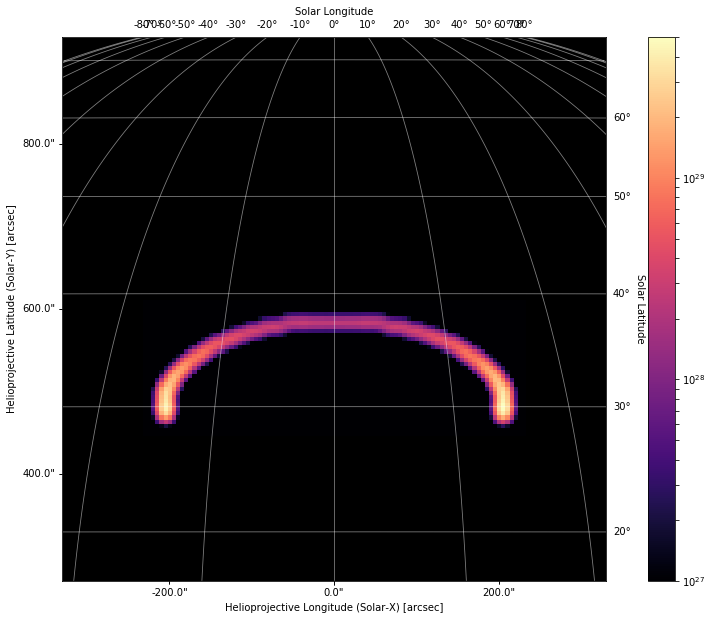
A commonly studied quantity in coronal loop physics is the emission measure distribution,
Notice that this quantity is computed by integrating along the line of sight from the observer to the feature on the Sun. That means we need both the density (which we computed above) as well as the location of the loop with respect to some observer.
Projecting and Binning#
Now that we have the loop coordinates and the density along the loop, we need to project the loop on the plane of the sky and integrate along the line of sight.
First, let’s choose an observing location. We can specify our observer using the same kind of SkyCoord object that we used to express our loop coordinates! We’ll place our observer at \((1\,\mathrm{AU},0^{\circ},0^{\circ})\), i.e. pointing right at the center of the Sun at a distance of 1 AU.
[9]:
observer = SkyCoord(lon=0 * u.deg, lat=0 * u.deg, radius=const.au, frame="heliographic_stonyhurst")
Next, we convert the loop to a Helioprojective coordinate system as defined by our observer.
[10]:
coords = loop.transform_to(Helioprojective(observer=observer))
To compute the line-of-sight emission measure, we’ll use a two-dimensional histogram and bin the \((\theta_x,\theta_y)\) coordinates, using \(n^2\Delta h\) as the weights. First, we need to set up the bins for our histogram.
[11]:
res_x, res_y = 5 * u.arcsec / u.pixel, 5 * u.arcsec / u.pixel
pad_x, pad_y = res_x * 5 * u.pixel, res_y * 5 * u.pixel
min_x, max_x = coords.Tx.min() - pad_x, coords.Tx.max() + pad_x
min_y, max_y = coords.Ty.min() - pad_y, coords.Ty.max() + pad_y
min_z, max_z = coords.distance.min(), coords.distance.max()
bins_x = np.ceil((max_x - min_x) / res_x)
bins_y = np.ceil((max_y - min_y) / res_y)
bins_z = max(bins_x, bins_y)
Next, we can compute the weights.
[12]:
dz = (max_z - min_z).cgs / bins_z * (1.0 * u.pixel)
em = density**2 * dz.value
We’ll exploit our helioprojective coordinate system to figure out what coordinates are blocked by the solar disk. First we need to figure out the angular size of the solar disk as seen by our observer.
[13]:
rsun_obs = ((const.R_sun / (observer.radius - const.R_sun)).decompose() * u.radian).to(u.arcsec)
Our loop will only be visible if it is in front of the disk or off the limb. Otherwise, we set it to zero visibility.
[14]:
off_disk = np.sqrt(coords.Tx**2 + coords.Ty**2) > rsun_obs
in_front_of_disk = coords.distance - observer.radius < 0.0
mask = np.any(np.stack([off_disk, in_front_of_disk], axis=1), axis=1)
[15]:
weights = em * mask
We can now use the histogram2d function in Numpy to bin our loop coordinates, weighted by the visible emission measure distribution, using the appropriate number of bins and ranges.
[16]:
hist, _, _ = np.histogram2d(
    coords.Tx.value,
    coords.Ty.value,
    bins=(bins_x.value, bins_y.value),
    range=((min_x.value, max_x.value), (min_y.value, max_y.value)),
    weights=weights,
)
We’ll also apply a Gaussian filter, with widths of 1 pixel in both directions, to simulate the point spread function of an instrument.
[17]:
em_hist = gaussian_filter(hist.T, (1.0, 1.0))
In order to make this into a sunpy.map.Map object, we also need to construct a header based on the observer location and the field of view of our observed loop.
[18]:
header = MetaDict(
    {
        "crval1": (min_x + (max_x - min_x) / 2).value,
        "crval2": (min_y + (max_y - min_y) / 2).value,
        "cunit1": coords.Tx.unit.to_string(),
        "cunit2": coords.Ty.unit.to_string(),
        "hglt_obs": observer.lat.to(u.deg).value,
        "hgln_obs": observer.lon.to(u.deg).value,
        "ctype1": "HPLN-TAN",
        "ctype2": "HPLT-TAN",
        "dsun_obs": observer.radius.to(u.m).value,
        "rsun_obs": ((const.R_sun / (observer.radius - const.R_sun)).decompose() * u.radian).to(u.arcsec).value,
        "cdelt1": res_x.value,
        "cdelt2": res_y.value,
        "crpix1": (bins_x.value + 1.0) / 2.0,
        "crpix2": (bins_y.value + 1.0) / 2.0,
    }
)
[19]:
em_map = GenericMap(em_hist, header)
Finally, let’s plot our loop emission measure!
[20]:
fig = plt.figure(figsize=(15, 10))
ax = fig.gca(projection=em_map)
im = em_map.plot(
    cmap="magma",
    title=False,
    norm=matplotlib.colors.SymLogNorm(1, vmin=1e27, vmax=5e29),
)
ax.plot_coord(SkyCoord(-300 * u.arcsec, 300 * u.arcsec, frame=em_map.coordinate_frame), alpha=0)
ax.plot_coord(SkyCoord(300 * u.arcsec, 900 * u.arcsec, frame=em_map.coordinate_frame), alpha=0)
em_map.draw_grid(grid_spacing=10 * u.deg, color="w", axes=ax)
ax.grid(alpha=0)
ax.set_facecolor("k")
fig.colorbar(im, ax=ax)
[20]:
<matplotlib.colorbar.Colorbar at 0x7f9e68aeeb00>
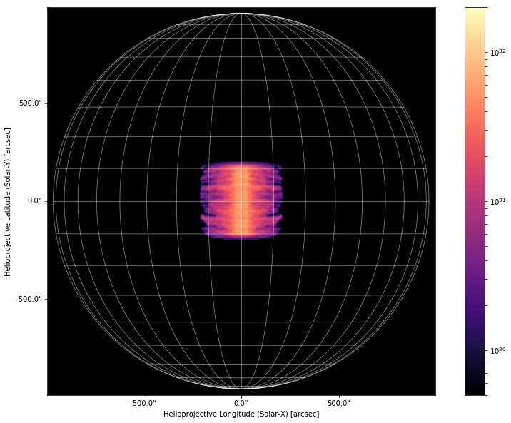
Extending to Many Loops#
One loop is not very exciting. Instead, let’s model an arcade of loops, choose their lengths from a power-law distribution, and place them over a range of latitudes.
Let’s write a function that generates the coordinates and densities for a lot of loops.
[21]:
def loop_arcade(n_loops, length_min=10 * u.Mm, length_max=100 * u.Mm, theta_min=-10 * u.deg, theta_max=10 * u.deg):
    # Generate loops
    rnd_gen = np.random.Generator(np.random.PCG64())
    x = rnd_gen.random(n_loops)
    alpha = -1.5
    lengths = ((length_max ** (alpha + 1.0) - length_min ** (alpha + 1.0)) * x + length_min ** (alpha + 1.0)) ** (
        1.0 / (alpha + 1.0)
    )
    thetas = np.linspace(theta_min, theta_max, n_loops)
    loops = [semi_circular_loop(l, theta0=th) for l, th in zip(lengths, thetas)]
    # Get densities
    ## Choose heating rate, get T from RTV scaling laws
    e = 1e-4 * u.erg / (u.cm**3) / u.s
    t = (1.83e3) * (e.value / 5.09e4 * (lengths.to(u.cm).value ** 2)) ** (2 / 7) * u.K
    density = np.hstack(
        [
            isothermal_density(loop, length, t=t.to(u.MK), n0=1e11 / (u.cm**3))
            for loop, length, t in zip(loops, lengths, t)
        ]
    )
    density = u.Quantity(density.value, "cm^-3")
    # Stack coordinates
    lon = u.Quantity(np.hstack([l.lon.value for l in loops]), loops[0].lon.unit)
    lat = u.Quantity(np.hstack([l.lat.value for l in loops]), loops[0].lat.unit)
    radius = u.Quantity(np.hstack([l.radius.value for l in loops]), loops[0].radius.unit)
    coords = SkyCoord(lon=lon, lat=lat, radius=radius, frame=loops[0].frame)

    return coords, density
[22]:
coords, densities = loop_arcade(
    1000, length_min=50 * u.Mm, length_max=500 * u.Mm, theta_min=-10 * u.deg, theta_max=10 * u.deg
)
Now that we’ve got the coordinates and densities for our arcade of loops, we need to bin them and convert them to a map. Let’s write another function that just encapsulates all of the steps that we walked through in the previous section.
[23]:
def arcade_to_map(coords, densities, observer):
    coords = coords.transform_to(Helioprojective(observer=observer))
    # Setup Bins
    res_x, res_y = 5 * u.arcsec / u.pixel, 5 * u.arcsec / u.pixel
    pad_x, pad_y = res_x * 5 * u.pixel, res_y * 5 * u.pixel
    min_x, max_x = coords.Tx.min() - pad_x, coords.Tx.max() + pad_x
    min_y, max_y = coords.Ty.min() - pad_y, coords.Ty.max() + pad_y
    min_z, max_z = coords.distance.min(), coords.distance.max()
    bins_x = np.ceil((max_x - min_x) / res_x)
    bins_y = np.ceil((max_y - min_y) / res_y)
    bins_z = max(bins_x, bins_y)
    # Compute Weights
    dz = (max_z - min_z).cgs / bins_z * (1.0 * u.pixel)
    em = densities**2 * dz.value
    rsun_obs = ((const.R_sun / (observer.radius - const.R_sun)).decompose() * u.radian).to(u.arcsec)
    off_disk = np.sqrt(coords.Tx**2 + coords.Ty**2) > rsun_obs
    in_front_of_disk = coords.distance - observer.radius < 0.0
    mask = np.any(np.stack([off_disk, in_front_of_disk], axis=1), axis=1)
    weights = em * mask
    # Bin values
    hist, _, _ = np.histogram2d(
        coords.Tx.value,
        coords.Ty.value,
        bins=(bins_x.value, bins_y.value),
        range=((min_x.value, max_x.value), (min_y.value, max_y.value)),
        weights=weights,
    )
    hist = gaussian_filter(hist.T, (1.0, 1.0))
    # Make header
    header = MetaDict(
        {
            "crval1": (min_x + (max_x - min_x) / 2).value,
            "crval2": (min_y + (max_y - min_y) / 2).value,
            "cunit1": coords.Tx.unit.to_string(),
            "cunit2": coords.Ty.unit.to_string(),
            "hglt_obs": observer.lat.to(u.deg).value,
            "hgln_obs": observer.lon.to(u.deg).value,
            "ctype1": "HPLN-TAN",
            "ctype2": "HPLT-TAN",
            "dsun_obs": observer.radius.to(u.m).value,
            "rsun_obs": ((const.R_sun / (observer.radius - const.R_sun)).decompose() * u.radian).to(u.arcsec).value,
            "cdelt1": res_x.value,
            "cdelt2": res_y.value,
            "crpix1": (bins_x.value + 1.0) / 2.0,
            "crpix2": (bins_y.value + 1.0) / 2.0,
        }
    )
    plot_settings = {"cmap": "magma", "title": False, "norm": matplotlib.colors.SymLogNorm(1, vmin=5e29, vmax=2e32)}
    return GenericMap(hist, header, plot_settings=plot_settings)
Let’s start by observing our arcade with the same observer that we defined in the previous section.
[24]:
arcade_map = arcade_to_map(coords, densities, observer)
[25]:
fig = plt.figure(figsize=(15, 10))
ax = fig.gca(projection=arcade_map)
im = arcade_map.plot()
ax.plot_coord(SkyCoord(-900 * u.arcsec, -900 * u.arcsec, frame=arcade_map.coordinate_frame), alpha=0)
ax.plot_coord(SkyCoord(900 * u.arcsec, 900 * u.arcsec, frame=arcade_map.coordinate_frame), alpha=0)
em_map.draw_grid(grid_spacing=10 * u.deg, color="w", axes=ax)
ax.grid(alpha=0)
ax.set_facecolor("k")
fig.colorbar(im, ax=ax)
[25]:
<matplotlib.colorbar.Colorbar at 0x7f9e68728400>
Looking straight at disk center is still a bit boring. Let’s choose a more interesting viewing angle by moving our observer to \((\Phi,\Theta)=(-25^{\circ},-25^{\circ})\)
[26]:
observer = SkyCoord(lon=-25 * u.deg, lat=-25 * u.deg, radius=const.au, frame="heliographic_stonyhurst")
arcade_map = arcade_to_map(coords, densities, observer)
[27]:
fig = plt.figure(figsize=(15, 10))
ax = fig.gca(projection=arcade_map)
im = arcade_map.plot()
arcade_map.draw_grid(grid_spacing=10 * u.deg, color="w", axes=ax)
ax.plot_coord(SkyCoord(-900 * u.arcsec, -900 * u.arcsec, frame=arcade_map.coordinate_frame), color="w", alpha=0)
ax.plot_coord(SkyCoord(900 * u.arcsec, 900 * u.arcsec, frame=arcade_map.coordinate_frame), color="w", alpha=0)
ax.grid(alpha=0)
ax.set_facecolor("k")
fig.colorbar(im, ax=ax)
[27]:
<matplotlib.colorbar.Colorbar at 0x7f9e681bed68>
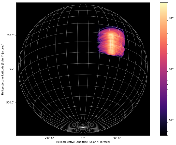
Note that we did not change our loop coordinates or the values of the densities. We only changed the location of the observer that defined our two-dimensional projected coordinate system.
The power of this approach is that our loop coordinates are independent of any one coordinate frame and we can define varying two-dimensional projections simply by varying the location of our observer. We don’t even need to think about transformation matrices, rotation matrices, etc. SunPy and Astropy provide all of this machinery for us!
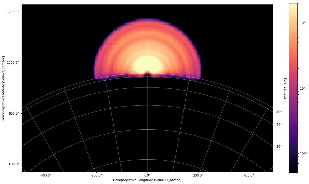
Let’s move our observer to the south pole such that we are looking through the arcade of loops.
[28]:
observer = SkyCoord(lon=0 * u.deg, lat=-90 * u.deg, radius=const.au, frame="heliographic_stonyhurst")
arcade_map = arcade_to_map(coords, densities, observer)
[29]:
fig = plt.figure(figsize=(18, 10))
ax = fig.gca(projection=arcade_map)
im = arcade_map.plot()
arcade_map.draw_grid(grid_spacing=10 * u.deg, color="w", axes=ax)
ax.plot_coord(SkyCoord(-450 * u.arcsec, 600 * u.arcsec, frame=arcade_map.coordinate_frame), color="w", alpha=0)
ax.plot_coord(SkyCoord(450 * u.arcsec, 1200 * u.arcsec, frame=arcade_map.coordinate_frame), color="w", alpha=0)
ax.grid(alpha=0)
ax.set_facecolor("k")
fig.colorbar(im, ax=ax)
[29]:
<matplotlib.colorbar.Colorbar at 0x7f9e686deb70>
We can even observe the loops off limb just by setting \(\Phi\ge90^{\circ}\).
[30]:
observer = SkyCoord(lon=-90 * u.deg, lat=0 * u.deg, radius=const.au, frame="heliographic_stonyhurst")
arcade_map = arcade_to_map(coords, densities, observer)
[31]:
fig = plt.figure(figsize=(18, 10))
ax = fig.gca(projection=arcade_map)
im = arcade_map.plot()
arcade_map.draw_grid(grid_spacing=10 * u.deg, color="w", axes=ax)
ax.plot_coord(SkyCoord(700 * u.arcsec, -300 * u.arcsec, frame=arcade_map.coordinate_frame), color="w", alpha=0)
ax.plot_coord(SkyCoord(1300 * u.arcsec, 300 * u.arcsec, frame=arcade_map.coordinate_frame), color="w", alpha=0)
ax.grid(alpha=0)
ax.set_facecolor("k")
fig.colorbar(im, ax=ax)
[31]:
<matplotlib.colorbar.Colorbar at 0x7f9e68173630>
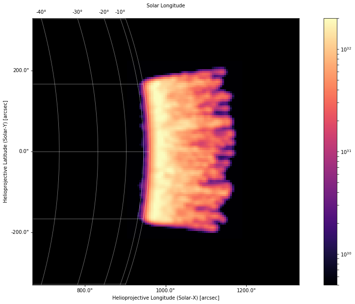
Notice that because of our viewing angle, the far footpoints are masked by the disk and thus are not visible.
Conclusion#
The sunpy.coordinates module can be a powerful tool for observers and modelers alike. Understanding how observed features on the Sun vary depending on the location of the observer is especially critical in the optically thin corona where many structures may be emitting along any given line of sight. Often it is difficult to disentangle distinct features in an observation and models become important in interpreting the underlying physics. Overall, the coordinates module in Astropy,
combined with the solar-specific coordinate frames in sunpy.coordinates, provide an intuitive and powerful way to express locations on the Sun in a frame-independent manner.